Synchronous Torque Model
Now the feasibility studies are done, the goal of the synchronous torque controller can be pursued.So the stepper code has been improved with a pre-emptive stepper algorithm.
This means we can include other pre-emptive code or drop this algorithm into the other code easily.
The motor control works fine at low speeds when using an external supply control (like a variable voltage switch mode PSU),
but when using the synchronous torque algorithm to start and at low RPMs the behaviour is chaotic.
So the solution may be to include a low frequency PWM algorithm (say 50Hz) to control the power delivered during the synchronous "mark".
This way the high power "kicks" the motor gets at low speeds are controlled by reducing the power of the pulses.
It would work, but it is moving away from the pure synchronous torque strategy which is key to reducing loss in the controller.
What needs to be achieved is the control of the motor should not be based on the sensors but an internal model of the rotation using the sensors to adjust the model.
This is sort of what the dq0 (clarke and park) model is doing, but dq0 requires ratiometric sensors, ADCs and complex maths algorithms, all of which cause delays in the processing.
The synchronous torque model is very fast partly because it uses digital sense information which requires no conversion.
This means the mechanics are a bit more complicated and the electronics also takes a hit too,
but the extra time and cost of this is offset by needing a faster CPU and ADCs to handle the analogue signals and authoring and debugging complex code.
There's also the issue of noise which means the ratiometric hall sensors cost quite alot more than digital ones and there is a compromise in accuracy.
All this is moving away from the strategy of using the simplest system as faster CPU, more complex code,
high speed ADCs and high accuracy ratiometric sensors are all effectively part of a hack to work around new problems introduced by going down this route.
This brings new problems which end up being a compromise, when a simple, accurate, well tested solution is already available.
The need for PWM proportional control will help in starting the motor from stationary and means the full power of the battery
will not be fed into the motor inductors to get the motor (and the car) moving, which was an issue.
Improved algorithms.
Added waveform analysis.

This are the core BLDC algorithms:
Using a Sampled PWM
This is where we have a PWM tick timer which is running at 50kHz (period 20uS).The PWM is timed by counting the number of 20uS ticks for each state (mark and space).
The sensor algorithm resets the state to space when the shaft moves to the next position.
This works better as there is no setting up and resetting of timer interrupts, which causes instability.
Also this means we can have a zero mark or space without confusing the CPU with a zero time interrupt.
Finally it means we can easily meter the amount of time the controller actually spends in a PWM state.
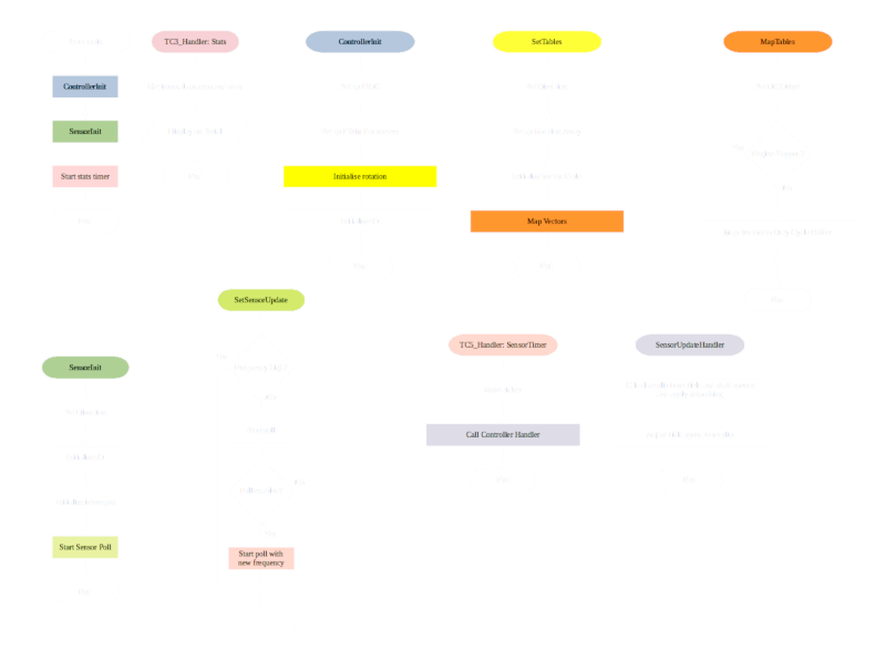
Here we have the core algorithms with the new sampled PWM algorithms:
These are (left to right):
- The PWM algorithm,
- The SYNCHRONOUSTORQUE version of the sensor algorithm and
- The low frequency PWM version of the sensor algorithm.
This is the PWM algorithm:
ISR (TIMER2_COMPA_vect)
{
    PWMUpdateTick++;

    if (PWMState == PWMINMARK)
    {
        if (PWMUpdateTick >= Mark) // Mark time expired, do space
        {
            if (Space > 0)
            {
                PORTB = 0;

                PWMState = PWMINSPACE;
            }

            PWMUpdateTick = 0;
        }
    }
    else if (PWMState == PWMINSPACE)
    {
        if (PWMUpdateTick >= Space) // Space time expired, do mark
        {
            if (Mark > 0)
            {
                ThisStep = PhaseMap (SenseIndex, Direction);

                PORTB = StepField[ThisStep];

                PWMState = PWMINMARK;
            }

            PWMUpdateTick = 0;
        }
    }
    else // Stopped
    {
        PORTB = 0;
    }
}
And this is the sensor algorithm:ISR (PCINT2_vect)
{
PortRead = PIND;
SensorRead = PortRead & SENSORMASK;
ReadPosition = SensorMap (SensorRead);
if (ReadPosition == NULLSENSE) // empty read
return;
SenseIndex = ReadPosition;
if (Mode == SYNCHRONOUSTORQUE)
{
// Restart as a space
PORTB = 0;
PWMUpdateTick = 0;
if (PWMState != PWMSTOPPED)
PWMState = PWMINSPACE;
}
else
{
// Continue mark in next step
if (PWMState == PWMINMARK)
{
SensorStep = PhaseMap (SenseIndex, Direction);
PORTB = StepField[SensorStep];
}
}
}
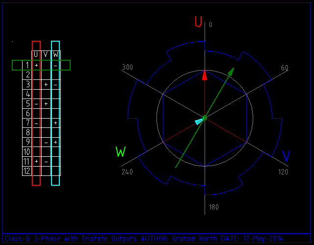
This using the runtime flag SYNCHRONOUSTORQUE to switch between the 2 algorthms.Also to understand how the motor is using the algorithms we need to see the fields acting in the motor.
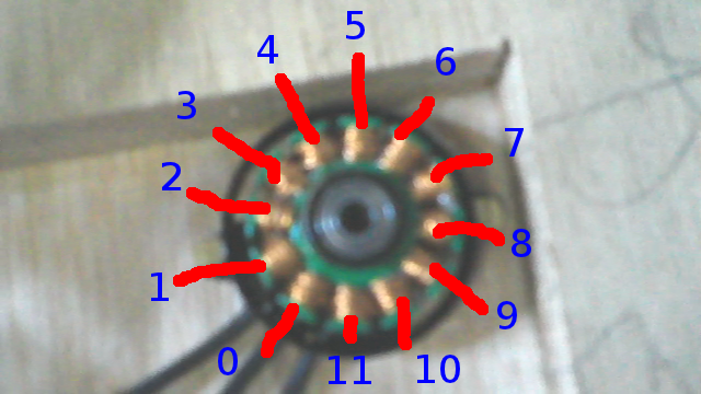
So the poles were assessed using a hall switch which stepping the fields.
Then these were put into an animation to see how it worked.
From this and other animations on this page the connectivity was worked out.
Also the fact that this is a DELTA motor, not a WYE as was expected.
        + + +                    11
       UUVVWW     01 23 45 67 89 01
       - - -     V  W  U  V  W  U  V
STEP1  010010     Ns    Ns    sN
STEP2  000110     Ns    sN    sN
STEP3  100100     Ns    sN    Ns
STEP4  100001     sN    sN    Ns
STEP5  001001     sN    Ns    Ns
STEP6  011000     sN    Ns    sN
                     Ns    sN    sN
                     Ns    sN    Ns
                     sN    sN    Ns
                     sN    Ns    Ns
                     sN    Ns    sN
                     Ns    Ns    sN
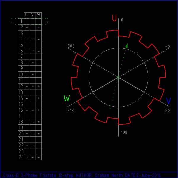
Class-D 3-Phase Controller Design
Having just read up about Class-D audio amplifiers, it appears there is the opportunity to simplify the design.This is a radical deviation in the design philosophy and requires modification of all parts of the controller.
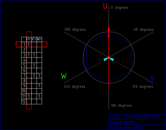
The Class-D amplifier is a H-bridge, or 2 x 180 degrees phases output.
This will be modified to a 3 x 120 degrees phases.
In the software, this means using a 3-output algorithm to drive to either rail instead of 6-output which control the rail switching independently.
Use the buttons below to see it work.
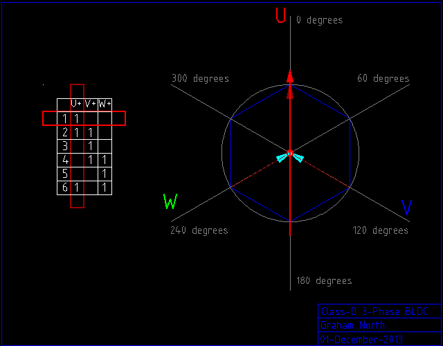
This is an animation of the class-D 3-phase algorithm.
Logic 1 sets a positive voltage and logic 0 sets a negative.
Also all the PWM phases must be phase aligned and zero output will be mapped to 50% mark/space ratio.
Obviously, this removes the possibility of shoot through.
Use the buttons below to see it work.
Software Flywheel SVM Model for AC synthesis
There is a way to have Space Vector Modulation without the heavy maths using a software flywheel model.This involves having an open loop SVM with sensor updates for the amplitude.
The open loop model rotates the stator field vector and thus the AC phase without sensor input.
The sensors interrupt and provide the position information as above.
The difference between the open loop model and the real position is calculated and this is used to adjust the scalar amplitude of the vector.
This scalar amplitude can be negative as the torque angle is 90 degrees, so less than 90 is positive and greater is negative.
This is better than DQ0 (clarke and park) since it does not rely on sensors to provide the vector.
The motor can continue to rotate even if there are no sensors.
Also there is an inherent delay in the calculation of DQ0 so there is an inaccuracy in that.
This is normally adjusted by calculating with a phase advance, but this is really just a guess as there is no way to predict the load.
Software flywheel model also can detect if there is a problem which DQ0 does not do naturally.
If the motor suddenly appears to do something impossible or dangerous (like suddenly reverse)
the comparison with the internal model will show this has happened and the controller can do something about it.
Arduino Timers and PWM
Arduino PWMs are run from the timers so they are independent of software.There are 3 timers each operate 2 PWM outputs giving 6 PWM outputs.
All 3 timers have different ways of configuring, but the common mode is 8-bit and they share a set of prescaler divisors.
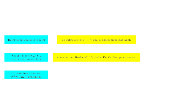
The trick is to set up the PWMs in the same mode and with the same prescaler, then reset all the timers and you will have all PWMs operating the same (including being in phase).
SVMController.git
Trigonometry Using 8-bit Integers
The ATmega328 CPU is an 8-bit integer CPU, so for the fastest performance the algorithms need to use this.The value 252 has common integer factors of both 3 (phases) and 4 (quadrants)
If the amplitude is -127 to +127 for full scale and the angles are calculated as 252 being a full turn this will work.
In pre-calculating a SINE table (which means fast trigonometry) only the first quadrant is needed.
all other quadrants can be calculated from this as with normal SINE,
however the values for a quarter/half/three-quarters/full turn are actually on quadrant boundaries.
This means to pre-calculate the first quadrant, values for 0 AND a quarter turn need to be included.
252 is a full turn, 252 / 4 = 63 so this means we need 64 values to include both the first (0) and last (63) values.
typedef struct
{
    signed char U;
    signed char V;
    signed char W;
}
PhaseAmplitudeSpec;

static const unsigned char SIN[64] =
{
      0,      3,      6,      9,     12,     15,     18,     21,
     24,     28,     31,     34,     37,     40,     43,     46,
     48,     51,     54,     57,     60,     63,     65,     68,
     71,     73,     76,     78,     81,     83,     85,     88,
     90,     92,     94,     96,     98,    100,    102,    104,
    106,    108,    109,    111,    112,    114,    115,    117,
    118,    119,    120,    121,    122,    123,    124,    124,
    125,    126,    126,    127,    127,    127,    127,    127
};

static const unsigned char MINUSTWOTHIRDSTURN  = 252 - (252 * 2 / 3);
static const unsigned char MINUSONETHIRDTURN  = 252 - (252 / 3);
static const unsigned char ONETHIRDTURN  = 252 / 3;
static const unsigned char TWOTHIRDSTURN = 252 * 2 / 3;

unsigned char AllQuadrantAmplitude (unsigned char Angle)
{
    if (Angle <= 62)
    {
        return SIN[Angle];
    }
    else if (Angle >= 63 && Angle <= 125)
    {
        return SIN[126 - Angle];
    }
    else if (Angle >= 126 && Angle <= 188)
    {
        return -SIN[Angle - 126];
    }
    else if (Angle >= 189)
    {
        return -SIN[252 - Angle];
    }
}

PhaseAmplitudeSpec AngleToAmplitudes (unsigned char Angle)
{
    unsigned char UAngle = Angle;
    unsigned char VAngle = 0;
    unsigned char WAngle = 0;

    signed char UAmplitude = 0;
    signed char VAmplitude = 0;
    signed char WAmplitude = 0;

    if (Angle < TWOTHIRDSTURN)
        VAngle = Angle + ONETHIRDTURN;
    else
        VAngle = Angle - MINUSONETHIRDTURN;

    if (Angle < ONETHIRDTURN)
        WAngle = Angle + TWOTHIRDSTURN;
    else
        WAngle = Angle - MINUSTWOTHIRDSTURN;

    UAmplitude = AllQuadrantAmplitude (UAngle);
    VAmplitude = AllQuadrantAmplitude (VAngle);
    WAmplitude = AllQuadrantAmplitude (WAngle);

    return {UAmplitude, VAmplitude, WAmplitude};
}

void ShaftMoveTick()
{
    ShaftAngle += ShaftSpeed; // Allow to wrap

    PhaseAmplitudeSpec PhaseAmplitude = AngleToAmplitudes (ShaftAngle);

    OCR0A = 128 + PhaseAmplitude.U;
    OCR0B = 128 + PhaseAmplitude.V;
    OCR1A = 128 + PhaseAmplitude.W;
}
The SINE table above is calculated for the first quadrant, but we need to calculate 0 to 63 inclusive (63 = exactly a quarter turn, so a quadrant boundary).
AllQuadrantAmplitude then will work correctly and produce accurate SINE values.
Also the angles for phase V and W need to be in the range 0 <= A < 252, which means in AngleToAmplitudes we need to allow for results which would be >252.
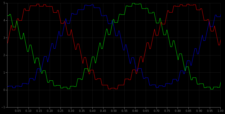
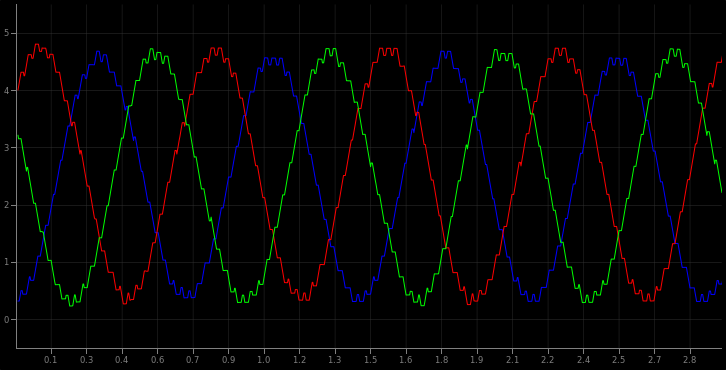
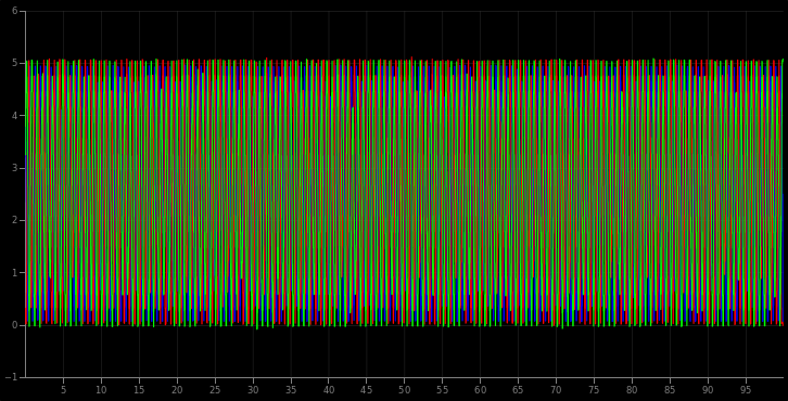
The waveforms for all 3-phases were output from the software to check the calculations:
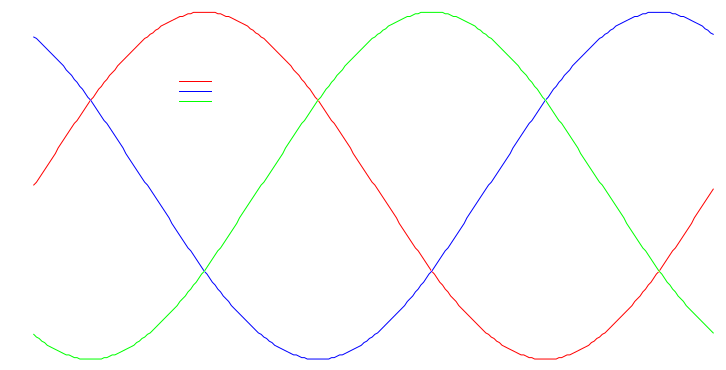
As you can see this is a very accurate 3-phase AC graph, which gives verification of the algorithms.
AC Amplitude Using 8-bit Integers
In order to factor the PWM Amplitude we need to be able to do fast divisionoutput = input * factor
...where 0 < factor < 1
In our case factor is not a value between 0 and 1, but 0 and 128.
So this means:
output = input * factor/ceiling
...where 0 < factor < ceiling and ceiling=128
So in reality:
output = input * factor / 128
or
output = (input * factor) >> 7
"Speed of math operations (particularly division) on Arduino" shows the multiplication of 8-bit integers is a 1 cycle operation (@16MHz 1 cycle = 62.5nS)
Instruction Cycles

MUL         2 (unsigned)
MULS        2 (signed)
MULSU       2 (signed with unsigned)

LSL         1
LSR         1
The number of cycles is for the full fetch-execute, but these are piplines, so multiplications are fast and so are bitshifts!
In order to do the "input * factor" bit we need a 16-bit answer to this might be a 16-bit operation.
According to all the documentation this is 6 times an 8-bit multiply so:
 6 * 62.5nS = 375nS for the multiply
 8 * 62.5nS = 500nS for the shifts
14 * 62.5nS = 875uS total
Maybe needs a bit more research, but this is a better solution than using tables.
PhaseAmplitudeSpec AngleToAmplitudes (unsigned char Angle)
{
    unsigned char UAngle = Angle;
    unsigned char VAngle = 0;
    unsigned char WAngle = 0;

    signed char UAmplitude = 0;
    signed char VAmplitude = 0;
    signed char WAmplitude = 0;

    if (Angle < TWOTHIRDSTURN)
        VAngle = Angle + ONETHIRDTURN;
    else
        VAngle = Angle - MINUSONETHIRDTURN;

    if (Angle < ONETHIRDTURN)
        WAngle = Angle + TWOTHIRDSTURN;
    else
        WAngle = Angle - MINUSTWOTHIRDSTURN;

    UAmplitude = AllQuadrantAmplitude (UAngle);
    VAmplitude = AllQuadrantAmplitude (VAngle);
    WAmplitude = AllQuadrantAmplitude (WAngle);

//output = (input * factor) >> 7
    return {
            (signed char)((UAmplitude * PWMAmplitude) >> 7),
            (signed char)((VAmplitude * PWMAmplitude) >> 7),
            (signed char)((WAmplitude * PWMAmplitude) >> 7)
           };
}

 . . .

void ADCReadComplete (unsigned char ADCIndex, unsigned short ReadValue)
{
 . . .
        switch (ADCIndex)
        {
            case 0:
                ShaftSpeed = ReadValue >> 2;
                break;

            case 1:
                PWMAmplitude = ReadValue >> 3; // 0 to 128
                break;

            default:
                break;
        }
 . . .
}
There is an offset due to integerisation so the standard maths rounding needs to be applied:
output = integer (input + 0.5)
0.5 is a floating point so this is done by bitshifting again:
(((UAmplitude * PWMAmplitude) >> 6) + 1) >> 1
Adding 1 before the last shift is the same as adding 0.5 to the result.
Also the scaling is actually 0 < factor < 127 -not 128
The PWM scales down gradually from the full scale by up to 1 count at 127 (max)
This is an average of 0.5, so adding 0.5 to the scale factor cures this:
ScalingFactor = PWMAmplitude + 0.5
This is done by bitshift and add again:
(((UAmplitude * ((PWMAmplitude << 1) + 1) >> 7) + 1) >> 1
This costs 2 more clocks for the add and extra shift.
 6 * 62.5nS = 375nS for the multiply
 8 * 62.5nS = 500nS for the shifts
 3 * 62.5nS = 125nS for the extra adds and shift
17 * 62.5nS = 1062.5nS ~ 1uS total
Double this to account approximately for the phase amplitude calculations and we are around 2uS for the whole thing.
at 6,500 rpm so 6500 * 4poles / 60seconds = 433.33 field rotations/second.
That's 0.002307692 secs or 2.3mS per rotation.
For at least a 6 step BLDC this means 2.3mS / 6 = 385uS at most for processing so that's no problem.
Each of the 252 steps of the full turn would take 0.000009158 secs or 9.158uS.
We need to calculate 3 phases so 2uS * 3 = 6uS.
This is safely less than the 9.158uS required to maintain maximum resolution at full speed.
A test of the real speed is required now.
Testing
A rather rough time testing of the update loop shows the calculations are a bit optimistic:ADCValueRead: [0]=3(1%) [1]=108(11%) [2]=120[3]=130[4]=141[5]=169(51A) ShaftMoveCount=45332 Update period 22059nS, shaft speed 2698 RPM ADCValueRead: [0]=0(0%) [1]=109(11%) [2]=117[3]=135[4]=159[5]=185(53A) ShaftMoveCount=45331 Update period 22059nS, shaft speed 2698 RPM ADCValueRead: [0]=0(0%) [1]=106(11%) [2]=120[3]=137[4]=164[5]=187(53A) ShaftMoveCount=45331 Update period 22059nS, shaft speed 2698 RPM ADCValueRead: [0]=4(0%) [1]=116(10%) [2]=125[3]=136[4]=160[5]=182(50A) ShaftMoveCount=45331 Update period 22059nS, shaft speed 2698 RPM ADCValueRead: [0]=5(0%) [1]=115(11%) [2]=122[3]=132[4]=144[5]=170(44A) ShaftMoveCount=45331 Update period 22059nS, shaft speed 2698 RPM . . .
Payload for flash is:
avrdude: writing flash (5342 bytes):
Also tested compiled with the O3 optimistion level (Os is default).
This did improve the time a bit:
SVMController, Jan  9 2014 (18:40:19)
ADCValueRead: [0]=7(1%) [1]=116(10%) [2]=97[3]=72[4]=37[5]=13(2A)
ShaftMoveCount=52922
Update period 18895nS, shaft speed 3150 RPM
ADCValueRead: [0]=4(0%) [1]=110(11%) [2]=105[3]=95[4]=74[5]=65(13A)
ShaftMoveCount=52321
Update period 19112nS, shaft speed 3114 RPM
ADCValueRead: [0]=0(0%) [1]=108(11%) [2]=114[3]=121[4]=121[5]=120(28A)
ShaftMoveCount=52313
Update period 19115nS, shaft speed 3113 RPM
ADCValueRead: [0]=7(0%) [1]=116(10%) [2]=121[3]=136[4]=162[5]=177(49A)
ShaftMoveCount=52298
Update period 19121nS, shaft speed 3112 RPM
ADCValueRead: [0]=5(1%) [1]=113(11%) [2]=120[3]=130[4]=145[5]=175(52A)
ShaftMoveCount=52300
Update period 19120nS, shaft speed 3113 RPM
 . . .
Payload for flash is:
avrdude: writing flash (6184 bytes):
So a 16% size increase for 15% performance improvement (ATmega328 flash size 32k).
Also attempted to explicitly optimise some of the maths operations:
SVMController, Jan  9 2014 (20:04:28)
ADCValueRead: [0]=17(1%) [1]=644(62%) [2]=643[3]=654[4]=673[5]=691(196A)
ShaftMoveCount=53304
Update period 18760nS, shaft speed 3172 RPM
ADCValueRead: [0]=16(2%) [1]=636(63%) [2]=648[3]=656[4]=675[5]=688(195A)
ShaftMoveCount=52668
Update period 18986nS, shaft speed 3135 RPM
ADCValueRead: [0]=7(1%) [1]=636(63%) [2]=646[3]=655[4]=668[5]=685(192A)
ShaftMoveCount=52667
Update period 18987nS, shaft speed 3134 RPM
ADCValueRead: [0]=16(1%) [1]=644(62%) [2]=642[3]=652[4]=670[5]=679(191A)
ShaftMoveCount=52672
Update period 18985nS, shaft speed 3135 RPM
ADCValueRead: [0]=17(2%) [1]=640(63%) [2]=646[3]=648[4]=659[5]=669(189A)
ShaftMoveCount=52668
Update period 18986nS, shaft speed 3135 RPM
 . . .
Also added further compilation optimisations:
SVMController, Jan  9 2014 (22:39:14)
ADCValueRead: [0]=212(20%) [1]=124(12%) [2]=116[3]=111[4]=99[5]=89(22A)
ShaftMoveCount=78089
Update period 12805nS, shaft speed 4648 RPM
ADCValueRead: [0]=207(21%) [1]=119(12%) [2]=126[3]=127[4]=140[5]=141(36A)
ShaftMoveCount=77162
Update period 12959nS, shaft speed 4592 RPM
ADCValueRead: [0]=205(21%) [1]=120(12%) [2]=127[3]=139[4]=156[5]=175(47A)
ShaftMoveCount=77150
Update period 12961nS, shaft speed 4592 RPM
ADCValueRead: [0]=213(20%) [1]=118(12%) [2]=127[3]=139[4]=160[5]=176(52A)
ShaftMoveCount=77147
Update period 12962nS, shaft speed 4592 RPM
ADCValueRead: [0]=211(21%) [1]=124(11%) [2]=122[3]=123[4]=133[5]=137(43A)
ShaftMoveCount=77151
Update period 12961nS, shaft speed 4592 RPM
Added code to differentiate time of the actual move algorithms, also refined the counter algorithms:
Fri Jan 10 14:04:19 GMT 2014
SVMController, Jan 10 2014 (14:04:15)
ADCValueRead: [0]=212(20%) [1]=116(12%) [2]=119 [3]=127 [4]=132 [5]=145(43A)
ShaftMoveCount=74889 LastMoveCount=0 TimeShaftMove=true
Update period 13353nS, this-last=13354nS, shaft speed 4457 RPM

ADCValueRead: [0]=207(20%) [1]=121(11%) [2]=114 [3]=112 [4]=106 [5]=107(33A)
ShaftMoveCount=500096 LastMoveCount=74890 TimeShaftMove=false
Update period 1999nS, this-last=-11353nS, shaft speed 5243 RPM

ADCValueRead: [0]=212(20%) [1]=119(12%) [2]=113 [3]=104 [4]=88 [5]=73(23A)
ShaftMoveCount=73574 LastMoveCount=500097 TimeShaftMove=true
Update period 13591nS, this-last=11592nS, shaft speed 5134 RPM

ADCValueRead: [0]=212(20%) [1]=124(11%) [2]=109 [3]=97 [4]=76 [5]=64(18A)
ShaftMoveCount=499964 LastMoveCount=73575 TimeShaftMove=false
Update period 2000nS, this-last=-11591nS, shaft speed 5135 RPM

ADCValueRead: [0]=210(20%) [1]=122(12%) [2]=113 [3]=103 [4]=83 [5]=74(19A)
ShaftMoveCount=73594 LastMoveCount=499965 TimeShaftMove=true
Update period 13588nS, this-last=11588nS, shaft speed 5136 RPM
The original calculated 6uS was for the AC synthesis calculations only.
There is other code involved in the ShaftMove loop which accounts for the other 5.6uS.
This was expected.
So as you can see we are looking at 11.6uS update speeds which equates to 5,135 RPM.
This is to maintain full accuracy of the 3-phase AC waveform.
For our 6,500 RPM giving 100 MPH, 5,135 RPM equates to 79 MPH.
1.29 angle ticks is 0.51% of a full field turn.
Or there are 195 updates per field turn.
On our Prius motor with 4:1 field to shaft this is 781 updates per rev (at full speed of 6,500 RPM)
So while it's not a perfect 3-phase AC waveform at full speed, it's certainly good enough.
Limitation of PWM in AC synthesis
Since we are using PWM and not an actual analogue output for AC synthesis this causes issues of it's own.The target PWM frequency is around 15kHz (we are actually testing at 32kHz) which is ~60uS period.
This means we can update the amplitude in 11.6uS but the PWM period is 60uS.
If the field rotation update period is 60uS we would have 252 * 60 = 15120 ~ 15mS rotation period.
1 / 0.01512 = 66.133 rotations/sec
...this is field rotations so 66 / 4 = 16.5 shaft rotations/sec.
16.5 * 60 = 990, so about 1,000 rpm.
If the designed speed is 100mph for 6,500rpm this means the vehicle will be going at 15 mph.
So to maintain precise AC synthesis the vehicle is limited to around 15mph,
which is much less than the limit due to update speed shown from testing above.
60uS / 2300uS (2.3mS per rotation) = 0.0261 rotations per PWM tick.
This means in the time it takes for a PWM output to go high then low the field has rotated over 9 degrees.
Or, put another way, this is 1/0.0261 = 38.3 PWM updates per rotation.
At these speeds the AC synthesis waveform would be inaccurate which leads to inefficiencies.
Compare that with Synchronous Torque where there is 1 update per sensor pass so:
6 sensors x 4 field rotations = 24 updates per rotation (and this is a fixed amount at all speeds).
The difference with Synchronous Torque is the updates are carefully timed to provide the most efficient torque pulse.
Whereas, with AC synthesis the updates are random in relation to the field.
The trade off between AC synthesis accuracy and PWM frequency would be true for all controllers, not just this one.
Higher frequencies would allow more accurate AC synthesis but at the cost of loss in the IGBTs.
Combined Hybrid Controller
I'm sure there are some clever phase compensating SVM algorithms for high speed AC synthesis,but our controller cuts to the chase by using the benefits of both AC synthesis and BLDC.
This would be the first controller of it's kind to do this.
BLDC is efficient at high shaft speed, but can be unstable at very low speed
due to the extremely short pulses needed to maintain momentum.
AC synthesis is smooth at low speed, but is less efficient at high speed due to inaccuracies in the waveform.
The aim is to use AC synthesis at low shaft speeds which gives us smooth control of the motor right down to stationary,
then at higher shaft speeds switch to BLDC to give us reliable pulsing up to the full speed of the motor.
SVM for AC synthesis would be done using the software flywheel and the BLDC would be the synchronous torque algorithm.
Obviously this means the transition between AC synthesis and BLDC would need to be carefully done.
The outputs are switched between PWM mode and direct output, and the field vector and amplitude would need to be smoothly maintained
The benefits over just AC synthesis would be more efficiency and higher power at higher shaft speeds.
Also this means the IGBTs would not need to deal with high frequencies at high power
so cheaper components can be used.
Sensor input
See also Digital Input ConversionSo we are using gray code to transfer the 6 sensors to a 3-bit binary input into the arduino.
Gray Code mapping:
| Gray Code | Decimal | Position Index |
|---|---|---|
| 000 | 0 | 7 |
| 001 | 1 | 0 |
| 011 | 3 | 1 |
| 010 | 2 | 2 |
| 110 | 6 | 3 |
| 111 | 7 | 4 |
| 101 | 5 | 5 |
| 100 | 4 | 6 |
The first and last positions are invalid, so the last position is 6 and the first position is 7.
In the software this needs converting back to an index, so a reverse gray code mapping is needed.
Reverse Gray Code mapping:
| Gray Code | Decimal | Position Index |
|---|---|---|
| 000 | 0 | 7 |
| 001 | 1 | 0 |
| 010 | 2 | 2 |
| 011 | 3 | 1 |
| 100 | 4 | 6 |
| 101 | 5 | 5 |
| 110 | 6 | 3 |
| 111 | 7 | 4 |
This is how it's implemented:
static const unsigned char GreyCodeIndex[] =
{
    7, 0, 2, 1, 6, 5, 3, 4
};

ISR (PCINT2_vect)
{
    PortRead = ~(PIND >> 2) & 0b111;

    SensorIndex = GreyCodeIndex[PortRead];
}

void ControllerInit()
{
// All pins set to output
    DDRB |= 0b00111111;
    DDRD |= 0b11100000; // Pin 2-4 as inputs

//-- Pin change interrupt on sensor inputs
    PCICR |= (1 << PCIE2);
    PCMSK2 |= 0b00011100;
Sensor Calibration
The angle relating to the index requires calibration.So code it added to do statistical analysis:
#ifdef SENSORTESTING
SenseRecordSpec SenseRecord[SENSORTESTING];

// Cumulative matrix of angle by position.
//  Stop at peak of 255
unsigned char SensorStatistic[252];
static unsigned char SensorStatisticPeak = 0;
unsigned char CurrentSensorStatistic = 0;
#endif // SENSORTESTING

 . . .

// Sensors (PORTD) interrupt
//  Fires each time the bit pattern changes
ISR (PCINT2_vect)
{
 . . .
# ifdef SENSORTESTING
 . . .

    if (SensorIndex == CurrentSensorStatistic)
        SensorStatistic[ShaftAngle]++;

    if (SensorStatisticPeak < SensorStatistic[ShaftAngle])
        SensorStatisticPeak = SensorStatistic[ShaftAngle];

    if (SensorStatisticPeak == 255)
    {
        memset (SensorStatistic, 0, 252);

        SensorStatisticPeak = 0;

        if (++CurrentSensorStatistic > 7)
            CurrentSensorStatistic = 0;

        if (CurrentSensorStatistic == 6) // Skip 6
            CurrentSensorStatistic++;
    }
# endif // SENSORTESTING
 . . .
}
#ifdef SENSORTESTING
static unsigned char LastSensorStatistic[252];
static unsigned char LastSensorStatisticIndex = 0;
static unsigned char SensorStatisticTickCount = 0;
#endif // SENSORTESTING

static inline void Stats()
{
 . . .
# ifdef SENSORTESTING
 . . .
            if (LastSensorStatisticIndex != CurrentSensorStatistic)
            {
                printf ("%u, %u, ", LastSensorStatisticIndex, SensorStatisticTickCount);

                unsigned char ShaftAngle = 0;

                for (; ShaftAngle < 252; ShaftAngle++)
                    printf ("%u,", LastSensorStatistic[ShaftAngle]);

                printf ("%u\n", LastSensorStatistic[ShaftAngle]);
                SensorStatisticTickCount = 0;
                LastSensorStatisticIndex = CurrentSensorStatistic;
            }
            else
            {
                memcpy (LastSensorStatistic, SensorStatistic, 252);
                LastSensorStatisticIndex = CurrentSensorStatistic;
                SensorStatisticTickCount++;
            }

# endif // SENSORTESTING
 . . .
}
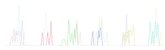
Which shows cumulative graph of the sensor hits by field angle.
0, 87, 0,0, ... ,0,0,13,106,138,36,36,151,252,125,25,17,84,136,52,5,0,0,0,1,0, ... ,0,0
1, 80, 0,0, ... ,0,0,10,126,116,17,2,37,197,226,84,110,251,154,101,65,60,32,32,83,121,49,12,0,0, ... ,0,0
2, 70, 0,0, ... ,0,9,105,102,20,1,8,139,252,72,67,123,47,3,0,0,0,0,0,1,0,1,0,0, ... ,0,0
3, 57, 0,0, ... ,0,0,10,99,79,5,6,97,160,253,216,131,89,12,0,2,51,91,47,2,0,0,0,0,0
4, 55, 0,0, ... ,0,0,12,99,70,7,74,231,254,173,53,98,59,5,4,64,95,23,2,0,0, ... ,0,0
5, 67, 0,0, ... ,0,0,1,11,94,100,56,120,122,212,252,119,95,124,60,8,9,71,103,42,5,0,0,0 .... ,0,0
7, 63, ... ,0,5,82,216,104,21,14,100,86,14,19,109,144,214,145,101,83,17,0, ... 0,0,8,71,138,109,81,22,41,102,67,8,72,162,254,155,121,80,8,0,0 ....
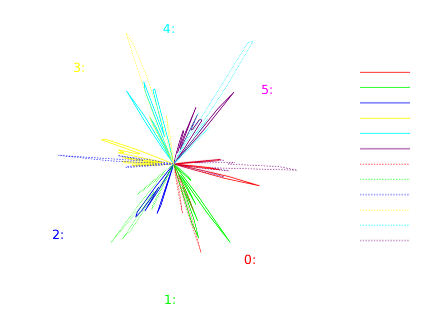
Which are compiled into some nice pretty graphs.
From this the average angle (which is assumed to be the shaft angle) can be assessed.
And this is added to the code, so now a closed loop algorithm is functional:
static unsigned char SensorAngle[] =
{
    92, 129, 169, 218, 4, 42
};

// Sensors (PORTD) interrupt
//  Fires each time the bit pattern changes
ISR (PCINT2_vect)
{
    PortRead = ~((PIND & 0b00011100) >> 2) & 0b111;

    SensorIndex = GreyCodeIndex[PortRead];

    signed short FieldAngle = SensorAngle[SensorIndex];

    if (Direction > 0)
    {
        FieldAngle += FIELDANGLE;

        if (FieldAngle > MAXANGLE)
            FieldAngle -= MAXANGLE;
    }
    else
    {
        FieldAngle -= FIELDANGLE;

        if (FieldAngle < 0)
            FieldAngle += MAXANGLE;
    }

    unsigned char i8FieldAngle = FieldAngle;

    UpdateField (i8FieldAngle);

    sei();
 . . .
}
Software Flywheel Algorithm
The sensor input only part of the story really.In order to have AC synthesis the zones between the sensor inputs are required.
This is where the "flywheel" comes in.
The angular velocity is calculated on a sensor update.
This is used to calculate angle updates based on time only without sensor input.
An unrefined test is added to assess the feasibility of the method.
This slow as it uses floating point variables and division, both of which are time intensive.
bool ShaftMoveTick()
{
 . . .
#ifdef SOFTWAREFLYWHEEL
    ShaftMoveTicks++;

    sei();

//  A = wt
    UpdateField (AngleWithWrap (LastFieldAngle, (unsigned char)((float)ShaftMoveTicks * AngularVelocity), 1));

#endif // SOFTWAREFLYWHEEL
 . . .
}

ISR (PCINT2_vect)
{
    PortRead = ~((PIND & 0b00011100) >> 2) & 0b111;

    SensorIndex = GreyCodeIndex[PortRead];

    unsigned char ThisFieldAngle = AngleWithWrap (SensorAngle[SensorIndex], FIELDANGLE, Direction);

    UpdateField (ThisFieldAngle);

    sei();
#ifdef SOFTWAREFLYWHEEL
    unsigned short TicksSinceLastUpdate = ShaftMoveTicks - LastShaftMoveTicks;

// w = A / t
// w = 42 / ticks
    AngularVelocity = 42.0 / (float)TicksSinceLastUpdate;

    LastFieldAngle = ThisFieldAngle;
    LastShaftMoveTicks = ShaftMoveTicks;
    ShaftMoveTicks = 0;
#endif // SOFTWAREFLYWHEEL
 . . .
}
To test the actual sensor field update was removed so the motor relies entirely on the time based updates.
The motor performed reasonably well at low speeds, but high speeds are just not working.
This is due to the inefficient algorithm.
None the less, the method works.
Next step is to redo the angular velocity algorthms with integer methods and no division.
This is going to require a bit of lateral thinking.
Floating point arithmetic without floating point
...and division without dividing
In a word: fractions.Floating point is a way of representing real, non-integer numbers.
Also it's a way of representing very large or very small numbers.
But there is another way and that is to use fractions.
The numerator and denominator are, of course, integers.
So we can represent a real non-integer number using two integers.
We can also have very small numbers where the denominator is large and the numerator is small.
Now, we are trying to represent a fractional increment of an angle (angular velocity)
so we can increment the field angle between sensor updates from a timer.
FieldAngle = AngularVelocity x Time

AngularVelocity = AngleDelta/TimeDelta

FieldAngle = AngleDelta/TimeDelta x Time
So rather than attempt to work with floating point we can implement an algorithm which uses the numerator and denominator directly:
bool ShaftMoveTick()
{
 . . .
    if (++ShaftMoveCounter >= Denominator)
    {
        FieldAngle = AddAngleWithWrap (FieldAngle, Numerator, Direction); // FieldAngle += Numerator .. or -= Numerator for reverse

        UpdateField (FieldAngle);

        ShaftMoveCounter = 0;
    }
 . . .
}
This counts the number of time ticks to stay on this angle (Denominator) then jumps the angle fraction (Numerator).
So for instance: 3/10 would be 10 ticks then move 3, or 1/5 would be 5 ticks then move 1.
All that remains is to calculate the fraction:
static inline void SensorChange()
{
 . . .
    AngleDelta = AddAngleWithWrap (FieldAngle, LastFieldAngle, -1); // AngleDelta = FieldAngle - LastFieldAngle
    TimeDelta = ShaftMoveTicks - LastShaftMoveTicks;

    Numerator = (((AngleDelta >> 4 ) + 1) >> 1);
    Denominator = (((TimeDelta >> 4 ) + 1) >> 1);
 . . .
}
We have the fraction from AngleDelta/TimeDelta but this would result in a jump of a whole sensor, in theory, which is pointless.
One sensor read is 1/6 of a turn which is 42 angle ticks,
so we "cancel" the fraction down by 32 using a math-rounding bitshift (in green above) which gives us close to 1 angle tick.
This was tested and works.
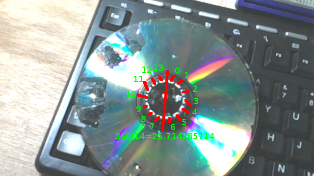
It produced relative stable rotation down to 60 RPM, and even as low as 25 RPM.
This is shaft rotations, so this is 2.167 field revs/second or 0.34 seconds/field rotation.
At these speeds, bearing in mind this is just a CD with small magnets so the torque would be very small.
Just the magnetic attraction when passing a sensor is enough to stop it.
In other words, slow enough for the momentum of the wheel to not be enough to carry it to the next sensor update.
So the software flywheel did carry the field to the next sensor smoothly.
Hybrid controller
HybridController.gitSince a working AC synthesis controller using the software flywheel is now developed, a hybrid AC synthesis/BLDC controller is the next step
This is a case of switching the PWM outputs to digital pin outputs, disabling the SVM algorithms and enabling the synchronous torque BLDC algorithms.
The design is to do this around 500 RPM but it may be more efficient at high power to do this a lower RPM.
First step is to integrate the BLDC code so it can be switched by key press.
Which is now done.
So we can use the software flywheel to improve the performance of the Synchronous Torque algorithm.
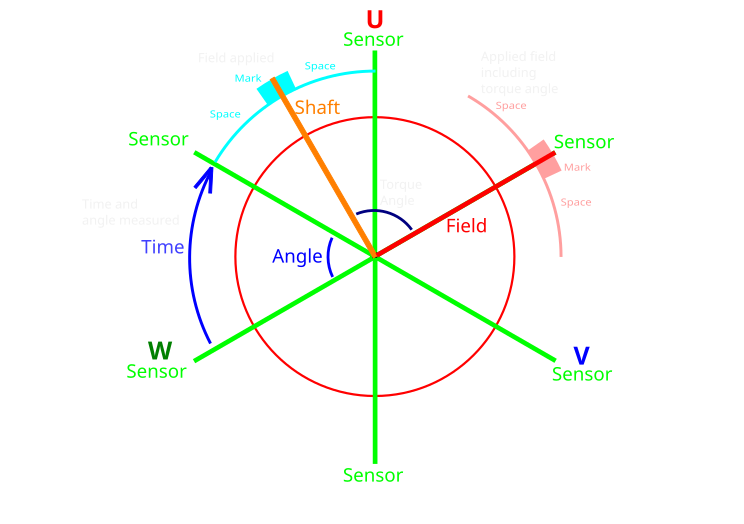
The torque angle applied is always 90 degrees.
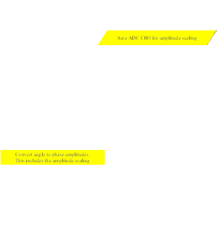
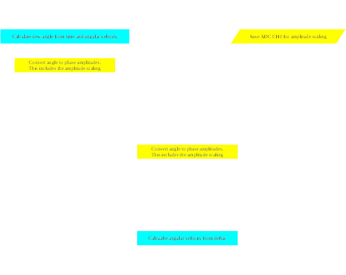
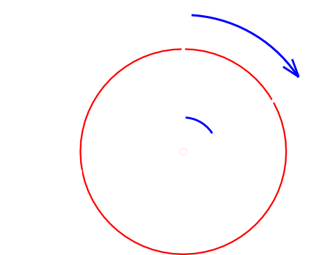
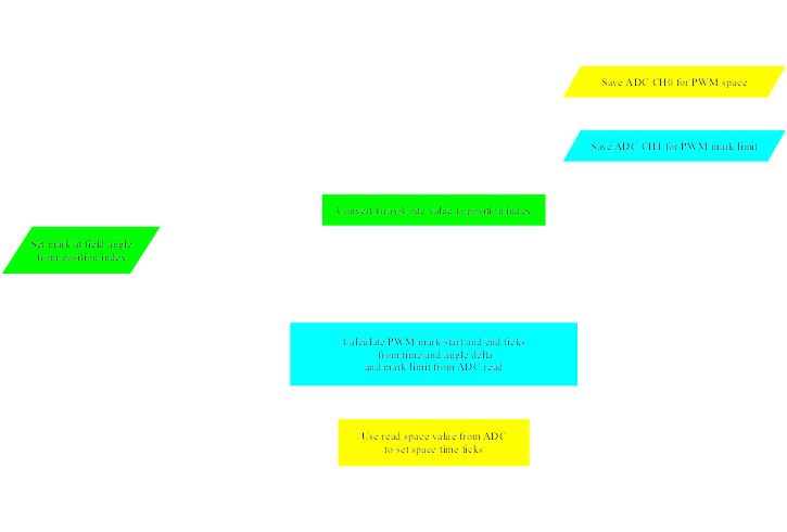
So the way it works is the angle is timed between 2 sensor updates (shown blue and orange).
This is used to time the software flywheel after the last update (orange) for the new sweep.
The field (red) is applied at 90 degrees to the shaft (orange) and timed for the "mark" to be in the middle of the sweep (pink).
Same as before the previous sensor updates will be used to assess the angular velocity and this will be use to calculate the mark position and width.
The algorithm will be much simpler as this does not have to calculate an angle fraction, just the time for the full step.
Trinary Logic Controller
Another way to operate the outputs, now the electronics are capable, is to use the third state of the pin.The pin can put into a open circuit (high impedance) state by setting it as an input.
This means the MCU output can be high(+), low(-) or open (blank) three distict states giving us trinary logic (also called ternary).
3-states corresponding to the states of the phases of the motor power lines.
It also mean the MCU can drive to all states without the possibility of shoot through.
Using trinary controller logic would be another industry first
Not to be confused with tri-state as that is simply using high impedance to allow multiple devices share a common bus.
This is using all 3 logic states of the MCU for actuating the output.
It is done using a binary CPU using the high impedance state of an input as the third state.
All current designs use either two separate binary outputs for the high and low side giving 4 states total,
or a single binary output, either high or low, with no off state (as with the Prius).
Use the buttons below to see it work.
Use the buttons below to see it work.
Latest version of UnoBLDC.cpp:
High Speed
Basically using assembler. This is the 1.3Mhz trinary PWM (50/50) to inspect the transitions:
.equ LOW_IN   = 0x00
.equ HIGH_OUT = 0xFF
.equ DDRB     = 0x04
.equ PORTB    = 0x05


    ldi	r24, LOW_IN
    ldi	r25, HIGH_OUT

loop:

;   nop equivalent to jump
;   nop
    out	DDRB,  r24; OFF

    nop
    out	PORTB, r24
    out	DDRB,  r25; LOW

    nop
    nop
    out	DDRB,  r24; OFF

    nop
    out	PORTB, r25
    out	DDRB,  r25; HIGH

    rjmp loop
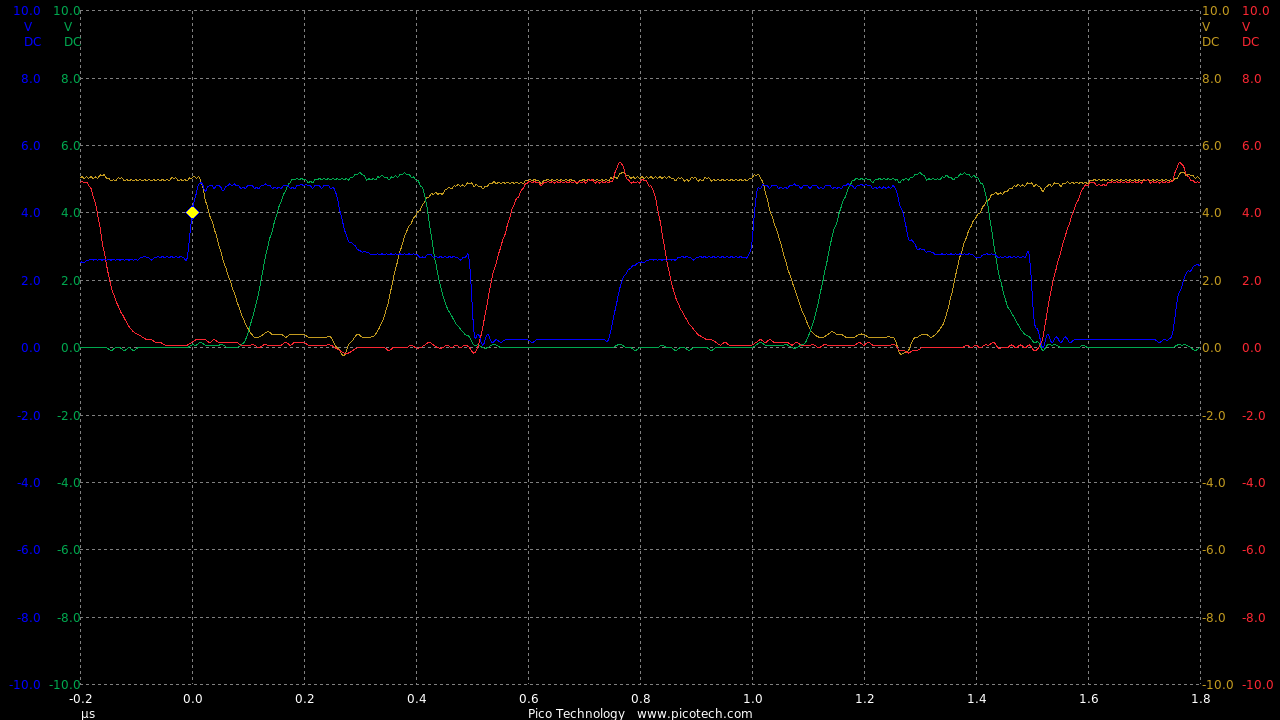
TIME:200nS/div, Blue:TP1(2vDC/div), Red:TP2(2vDC/div), Orange:TP3(2vDC/div), Green:TP4(2vDC/div).
This is showing fast transitions for high (Green) and low (Red) with the max wait 100nS and max switch 100nS.
Which means the total switching delay is 200nS well within the 1uS required.
Latest Tesla version of trinary.asm:
This produces a 1.33MHz trinary waveform with 50/50 mark/space on an Arduino Uno.
It was mainly done to test the electronics.
So if we want this to be used, in theory we can have a 1.33MHz / 128 = 10.42kHz trinary with full sine wave SVM.
Which, while inside the human hearing is quite acceptable.
SVM frequency
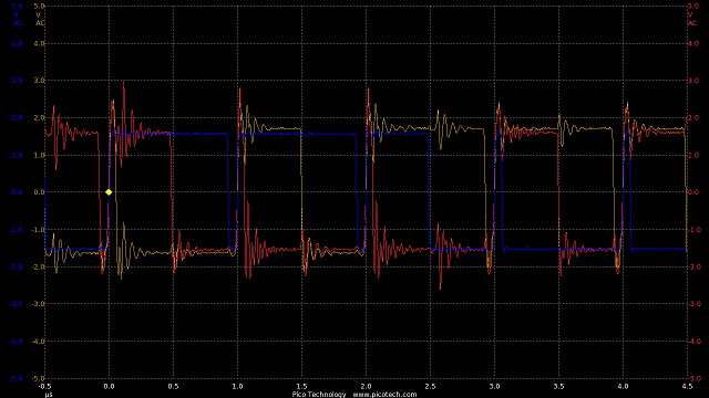
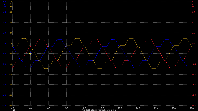
Probing the outputs to see the real synthesised 3-phase.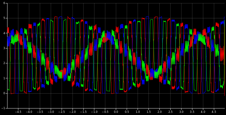
This is running at a rotational frequency of about 1700Hz
The wheel circumference is approx 2m, the gearbox is 9.73:1 and there is a 2:1 field to shaft in the 4-pole motor.
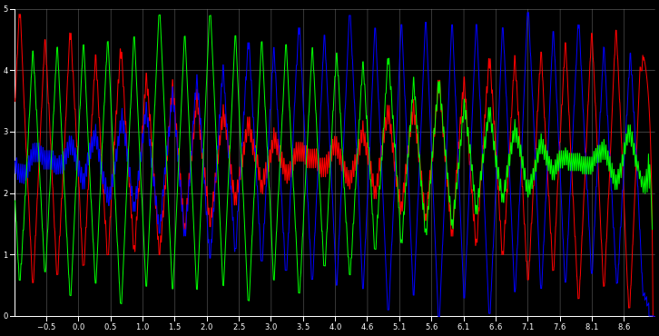
This is running at a rotational frequency of 2.5kHz which is the highest frequency the software will currently run
If it were possible this would over 500mph
This is the same but at a higher update frequency
..and 1333Hz which would be around 300mph
..and the same output over 0.1 seconds
This means in all realistic speeds it's a good approximation of 3-phase.
ADCValueRead: [0]=1023(100%) [1]=1023(100%)
Numerator=17 Denominator=1 AngleDelta=0 ReadCount=0 FieldTurnCount=0 Revs/sec=0 RPM=0 PWMAmplitude=127 ShaftSpeed=144
IdleTime=0
Arduino Due SVM
As it turns out the SAM3X chip used in the Arduino Due was designed with motor controllers in mind.It's not just that the CPU has 5 times the clock speed (84MHz), but also the waveform synthesis is hardware accelerated.
These devices are capable of producing 3-phase AC synthesis at over 100kHz.
On Arduino Due PWM, ard_newbie shares some demo code for it.
There are some bugs with this persons code, but it is a good basis for using the accelerated hardware.
Here is a 1MHz PWM (500nS/div):
..and synthesising 167kHz AC 3-phase waveform (2uS/div with real-time smoothing of the above):
This is 2 orders of magnitude higher than the requirements of AC synthesis and well beyond the capabilities of all high power IGBTs,
but demonstrates the amazing capabilities of this low-cost CPU.
Other projects:
https://github.com/collin80/DueMotorCtrl also based on the Arduino Due
https://github.com/MPaulHolmes/AC-Controller based on the MicroChip dsPIC30F4011
Ethernet on Arduino
The communication between the controllers and the display in the car are going to be using good old ethernet.It's much faster than CAN bus and it means a person can diagnose the problems on a PC without any special hardware, like ODB-II units.
And the USB-serial communication is quite simple and very useful, but it just doesn't cut it when you need high speeds for real time displays.
- LIN: 19.2kbps.
- USB serial: 112kbps (up to ~1Mbps if you use a special serial module).
- USB 2.0: 480Mbps.
- CAN: up to 8Mbps, but that's stretching the limit. Most chips operate at 10-100kbps.
- SPI: as a defacto standard effectively unlimited. Chipset with 100Mbps are not uncommon.
- Ethernet: 10Gbps is currently used for server interconnects (although the W5100 chip is only capable of 25Mbps).
As ever this means we need to author some simple core code which will do what we need without the Arduino libraries.
The libraries are good, for what they are, but when I'm packing in all the controller functionality
and ensuring it runs smoothly without lockups this needs quite a bit of refining.
Including dealing with SPI and the SPI protocol and using external interrupts on the Arduino
The arduino ethernet shield uses a Wiznet W5100 chip (datasheet | notes)
SRAM Diets
It seems the SRAM of the Arduino was getting eaten up by constant data, which should not happen in a flash based device.Further research shows that although 'const' is added to all the static data, it is still placed in the SRAM.
In order to leave this in flash there is a pgmspace module with macros and constants for referring to data in flash.
Part of the reason for this is the Harvard architecture, which runs program instructions from 16-bit Flash and has program data in 8-bit SRAM.
The flash and SRAM are actually connected to different busses so the CPU can fetch from both flash and SRAM at the same time.
It doesn't take a genius to see how this would make the system run much faster.
So in order to access constant data held in flash (which is not a data area) we need special instructions.
The LPM assembly instructions are 3 clock cycle instructions so there is a hit on performance,
but this means you can store large tables so reducing calculation times.
Also long text strings for debugging can be stored there giving meaningful output rather than cryptic error codes.
PWM Testing
See also: HV Power LabLatest version of Trinary.cpp:
Van Controller
For the simple PWM controller in the van, this just initially using the PWM stuff in the Arduino.Also reading the keyboard inputs to change the modes for testing and some fixed "control" inputs.
Latest ethernet version of UnoTest.cpp:
An ADC external multiplexer is added to the electronics so this needs the software to do this.
Also now the software is reading a pulse sensor on the motor shaft it needs to be able to use PIN interrupts
and probably a real-time clock of some description.
The real-time clock can be done in a minimal way with a timer interrupt increment a variable which is reset with each update.
Some experiments were added to this for the ethernet, but there was something unstable about the client.
There is an issue with NC not transmitting key presses (it only transmits after hitting return), so a client was built which does this.
Latest ethernet version of TCPClient.cpp:
Since the van controller is actually not Arduino hardware, but the AVR chip mounted in the PCB of the controller,
there is no ability to add a shield so this may not be included.
Latest version of UnoTest.cpp:
The power train for the van is being completed making the van a usable vehicle from the electronic sense
The vehicle moving (with fixed PWM at 100Hz)
Synchronous Current Sensing
Since the current input is sampled and the sample rate depends on the ADC read time (plus other things) it is arbitrary as to whether this will read when in mark or space.This problem is a by-product of using a low freqeuncy PWM since the mark and space are so long the current reading might well occur when in a space and be artificially low.
What is actually happening is the current reading is a modulated interference with the PWM sample.
To fix this the current is read as soon as possible after the mark starts using the interrupt from the timer which controls the PWM.
From observation and using a calibrated current meter the software sees a current value roughly half the meter, so a factor of 2 is used to compensate.
AC Induction Control
AC induction motors are controller by setting the field rotational speed to be above the rotor shaft speed.
This is simply done by sampling the speed of the shaft and setting the field rotational speed to set the slip.
Every 20ms the slip is calculated by the controller and the field speed is adjusted to retain the slip.
The pedal input sets the amplitude; high amplitude reduces the slip, so the ACIM algorithm increases the field speed to retain the slip.
If the amplitude is reduced the ACIM algorithm decreases the field speed in line with the shaft speed.
It's done this way so the user input (via the pedal) directly controls the torque of the motor and simplifies the ACIM algorithm.
This way the ACIM algorithm is fast and the control is very responsive.
PIC software created in Piklab, Arduino software created in the Arduino IDE, animations created in qcad/librecad, plots and graphs GNumeric and SciLab, images edited in gimp, flowcharts created in LibreOffice Draw.